Statistics & ML Concepts for your Next Quant Finance Interview

Statistics and machine learning are two concepts that tend to be quite prevalent in quantitative finance interviews. While the degree to which these concepts are assessed may vary depending on whether you are pursuing a quantitative research, trader, or developer role, knowing the foundations can help ensure that you are prepared in the case that they appear.

In this article, we'll cover six fundamental concepts in statistics and machine learning and we'll provide examples of how they're used in practice. If you're interested in finding some practice statistics interview questions, check out our article on stats interview questions.

1. Metrics to Evaluate a Classification Model

When evaluating a classification model, it may initially seem like using accuracy is the best choice. However, if our data is imbalanced (one class is more prevalent than the other) there are many other metrics that one should also consider.

• Precision: Refers to how well the model performs when it predicts a positive outcome. Mathematically, this can be expressed as:

  (Number of True Positives) / (Number of True Positives + Number of False Positives)

  Precision tends to be a good metric to consider when the risk of a false positive is very high. For example, in the case of spam detection, we wouldn’t want to accidently classify an important email as spam as the recipient of the email may miss the message.

• Recall: Refers to how well the model predicts positive outcomes. Mathematically, this can be expressed as:

  (Number of True Positives) / (Number of True Positives + Number of False Negatives)

  Recall tends to be a good metric to consider when the cost of a false negative is very high. For example, in the case of cancer detection, a false negative would mean that the patient wouldn’t be recommended to receive treatment which would be detrimental to their health.

Like many other concepts in statistics, precision and recall have a tradeoff. Increasing precision, often comes at the expense of reducing recall. This tradeoff can often be seen through the ROC curve. The ROC curve plots the true positive rate against the false positive rate for different thresholds. We want this curve to extend to the top left and we want to maximize the area under the curve.

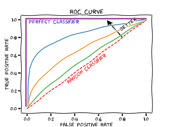
Often, our goal is to maximize the true positive rate while minimizing the false positive rate. One way to think about this is that we can increase our true positive rate simply by predicting more observations to fall under the “positive class”. This way we’ll catch all the true positives. However, by increasing the flexibility by which we classify observations as positive, we also increase the probability that we accidently classify a “negative” sample as “positive” (this is called a false positive). Therefore, we want to capture the true positives, but we don’t want to do so to the point that we also always incorrectly classify negative samples as positive. Now, there may be situations in which we are ok with falsely classify some observations as positive, as long as we do capture all positive observations. The great part about the ROC curve is that it lets us observe what thresholds we can set to align with this objective.

2. Linear Regression

Linear regression is a supervised machine learning method that predicts a dependent variable based on a set of independent variables. Our goal is to find the coefficients that fit the data as best as possible in order to minimize the residual sum of squares (the sum of the squared differences between the prediction of the linear regression model and the true value). In the simple linear regression case we have an intercept B0 and a slope term B1, which represents the change in the response for every 1 unit increase in X. Linear regression comes with many assumptions. We outline these assumptions below:

1. Linearity of the predictor-response relationship

2. No correlation between the error terms (the error terms are independent)

3. A constant variance of error terms (homogeneity of variance)

4. Normality of the error terms (the error terms follow a normal distribution)

5. No multicollinearity

We can check whether conditions 1 to 3 hold by plotting the residuals against the fitted values. In this plot, we want to ensure that there are no visible patterns that may indicate a violation of our assumptions. We can check condition 4 by conducting the Shapiro-Wilk test, which tells us how close the sample data fits a normal distribution, or by creating a q-q plot. Finally, we can check condition 5 by calculating the variance inflation factor (VIF). Oftentimes, a value ≤ 10 is considered ok. Since linear regression is a parametric model (it can be defined explicitly by a function), it can often suffer from underfitting and have a high degree of bias in its predictions. If you’re interested in learning about more ways to improve linear regression you can look into polynomial regression, regularization, and subset selection.

3. K-Means Clustering

K-Means clustering is a unsupervised machine learning method that takes as input a dataset and segments that dataset into multiple groups. This algorithm is called “unsupervised” because it isn’t provided labels (the response variable) during the training process. The model begins by partitioning the data into K clusters and then arbitrarily selects centroids for each of these clusters. The remaining points are assigned to the cluster that is closest to them, often defined by Euclidean distance, and then the centroids are updated by calculating the mean of each group that is formed. This process is repeated until the algorithm converges - meaning no more iterations will change the groupings that are formed.

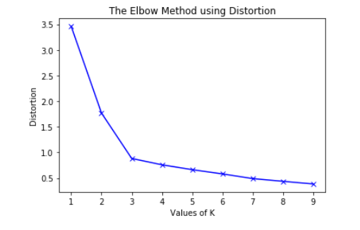
With K-Means, we are allowed to select a parameter K, that controls the number of clusters that will be created. One common method for selecting the best value of K is the elbow-method. The idea here is that the first few clusters will explain the majority of the variation seen in the data. By plotting the explained variation as a function of K, we can see at what point increasing K no longer leads to a decrease in the unexplained variation in the data. See the chart below for more details.

4. Random Forests

Random Forests are an ensemble machine learning technique that can be used in both the regression and classification setting. Ensemble methods leverage the combination of multiple models in order to improve predictions. Random Forests in particular, use Decision Trees as the models that they combine. Decision trees in the classification setting make splits to maximize the information gain, while decision trees in the regression setting perform splits to minimize the mean squared error. Individual decision trees are very prone to overfitting, so random forests attempt to eliminate this issue through the use of bagging or boosting.

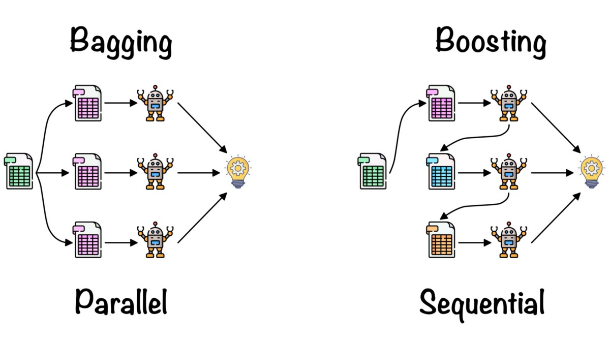
1. Bagging is an ensemble technique in which multiple weak learners learn independently, and their predictions are combined by taking the average.

2. Boosting is an ensemble technique in which weak learners build on top of each other, with each new learner improving the predictions of the previous learner.

If you’re interested in learning more about bagging and boosting check out "adaptive boosting” and “gradient boosting”.

5. Principal Component Analysis

PCA is a very popular dimensionality reduction technique that reduces the number of features in our dataset. The goal of PCA is to summarize a set of variables with a smaller set of representative variables that explain most of the variability in the original set. This is often used to counteract the effects of overfitting by reducing model complexity. It also helps to solve the “curse of dimensionality”, which refers to the situation where the amount of available data is too little in comparison to the dimensionality of the feature space. Furthermore, PCA can also be used as a data visualization technique to view high-dimensional data in two dimensions.

There are two popular methods for principal component analysis: normal PCA and incremental PCA. Normal PCA is the default algorithm that is often employed and works for datasets that can fit in memory. When the dataset can’t fit into memory we often use Incremental PCA.

One way that we can evaluate whether PCA is effective in our scenario is by fitting a machine learning model using the principal components, measuring the new performance, and comparing the performance back to the model that incorporated all the features. Ideally, we would like to see a similar performance between the two models. Since our goal with PCA is to reduce the number of features while still explaining a significant amount of the variability in the data, a similar performance would indicate that PCA is effective here.

6. Cross-Validation

Cross validation is a technique used to evaluate the performance of a machine learning model in terms of how well it will generalize to new data sets. There are multiple methods for performing cross validation and here we’ll walk through a few of them.

1. Validation Set Strategy

   In this strategy, we divided the set of observations into a training set and a validation set. The model is fit on the training set, and its performance is evaluated on the test set. The cons of this approach are

   • The validation error can be highly variable depending on the randomly generated train and validation data sets.

   • The validation error may overestimate the test error because it could have been trained on so few samples (i.e the training data set was too small)

2. Leave-one-out Cross Validation (LOOCV)

   In LOOCV, a single observation is used for the validation set, and the remaining observations make up the training set. In other words, if we have n observations, n-1 will be used for training and 1 will be used for validation. This procedure is repeated n times to get n squared errors and the resulting LOOCV is the average of these errors. The pros of this approach are:

   • There is far less bias in the result when compared to the validation set strategy 2. We are not limited in the amount of data we can use to train the model.

   • The cons of this approach, however, are that the procedure has to run n times and therefore can often be computationally infeasible for very large data sets.

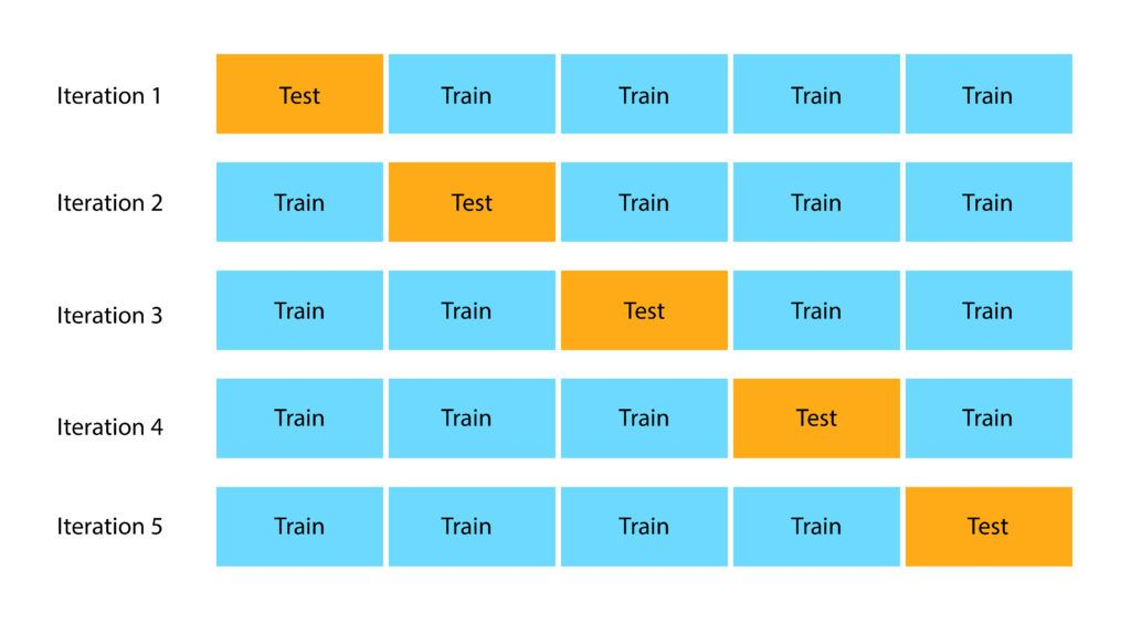
3. K-Fold Cross Validation

   In K-Fold CV we randomly divide the groups into K-folds of approximately equal size. The first fold is treated as a validation set, and the model is fit on the remaining K-1 folds. We repeat this procedure K times. In each repitition we rotate which fold is used for the validation set. The result is k errors which are averaged to get the CV score. The advantages of this approach are that

   • Much more computationally feasible

   • More accurate test error estimates because there is less overlap in the training sets on each run of the procedure.

Closing Remarks

Thanks for checking out this article on stats/ml concepts for the quant finance interview. If you're looking to land your next job or internship in quantitative finance check out OpenQuant. You'll find the best, and most relevant, roles from some of the top companies in the quantitative finance industry. Also, if you enjoyed this blog, feel free to read more of our content by clicking the button below.